Intro

We would like to train, validate and test some models by doing parameters tuning. In order to archieve it, the dataset will be splitted in a train set, a validation set and a test set. The second one will be used to evaluate the model with a different set of k/hyperparameters in order to choose the set of parameters that gives the highest accuracy on the validation set. After the tuning on the validation set has been done, we will check the performance of our model on the test set.

Dataset and preprocessing

Once we have loaded the Wine dataset, we could use some dimensionality reduction technique, but we just take the first two features of the dataset and discard the other ones (applying a PCA reduction at 2 dimensions using all the features available could gain a lot the prediction result, because instead of losing a lot of information by discarding the other features we could limit the loss by projecting all the features in a max-variance plane).

Then the dataset will be shuffled and splitted into train (50%), validation (20%) and test (30%) sets.

X, y = datasets.load_wine(return_X_y=True       
X = X[:, 0:2]
X_trainval, X_test, y_trainval, y_test = train_test_split(X, y, test_size=0.3,random_state=1)
X_train, X_val, y_train, y_val = train_test_split(X_trainval, y_trainval,test_size=0.2857, random_state=0)

Preprocessing is the foundamental task, so once we have splitted the three sets, it is time to normalize. If we normalize every set, we leak information about either the response (from the future, from our hold out data set into the training) or the evaluation of our model. This can cause considerable optimism bias in our model evaluation. The idea in model validation is to mimic the situation we would be in when our model is making production decisions, when we do not have access to the true response. The consequence is that we cannot use the response in the test set for anything except comparing to our predicted values.

Another way to approach it is to imagine that we only have access to one data point from our hold out at a time (a common situation for production models). Anything we cannot do under this assumption we should hold in great suspicion. Clearly, one thing we cannot do is aggregate over all new data-points past and future to normalize our production stream of data, so doing the same for model validation is invalid. We don’t have to worry about the mean of our test set being non-zero, that’s a better situation to be in than biasing our hold out performance estimates. Though, of course, if the test is truly drawn from the same underlying distribution as our train (an essential assumption in statistical learning), said mean should come out as approximately zero.

But in this case we will not normaliza, as we are analyzing a really reduced and not-so-dispersed dataset.

K-nearest neighbor

k-NN is one of the most easy algorithms for ML classification/regression. An new object is clas- sified on the majority vote from the k nearest neighbors. The parameter k is odd (in binary classifications it could happen some parity situation), it must be tuned and it depends on the dataset. Generally, for an increasing k the noise which compromises the classification decreases, but the criterion of choice for the class becomes more blurred. The choice can be made through heuristic techniques such as cross-validation. For what concerns our case, we will:

• Train on the train set.
• Evaluate for k=1, k=3, k=5 and k=7.
• Choose the best model 4. Apply it on the test set.

Model training and evaluation

In order to train the models we instantiate a KNeighborsClassifier for for each k (n_jobs set to -1 forces the program to use the maximum cores available on the running machine, since this classifier is as simple as computational intensive) and we fit on the train set. At the same time we use the model to predict on the validation set and we save everything in a data structure and, using a personal library, we plot the four models with the decision boundaries.

print("\n********************************")
print("TASK: kNN classification")
print("********************************\n")

best_score = 0
best_k = 1
knn_models = []
knn_accuracies = []
for k in [1, 3, 5, 7]:
knn = KNeighborsClassifier(n_neighbors=k, n_jobs=-1)
knn.fit(X_train, y_train)

knn_models.append(knn)
accuracy = knn.score(X_val, y_val)
knn_accuracies.append(accuracy)
if accuracy > best_score:
  best_score = accuracy
  best_k = k

print('Best prediction accuracy on validation set found with k = ' + str(best_k))
print('{:.2%}\n'.format(best_score))
plotModels(fignum=0, X=X_train, Y=y_train, models=knn_models, titles=[
'k=1', 'k=3', 'k=5', 'k=7'], n=2)
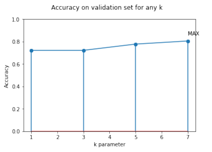
plotAccuracyComparison(fignum=1, the_list=[1, 3, 5, 7], accuracy_list=knn_accuracies, x_label='k parameter', title='Accuracy on validation set for any k', type='linear')

TASK: kNN classification

Best prediction accuracy on validation set found with k=7 -> 80.56%

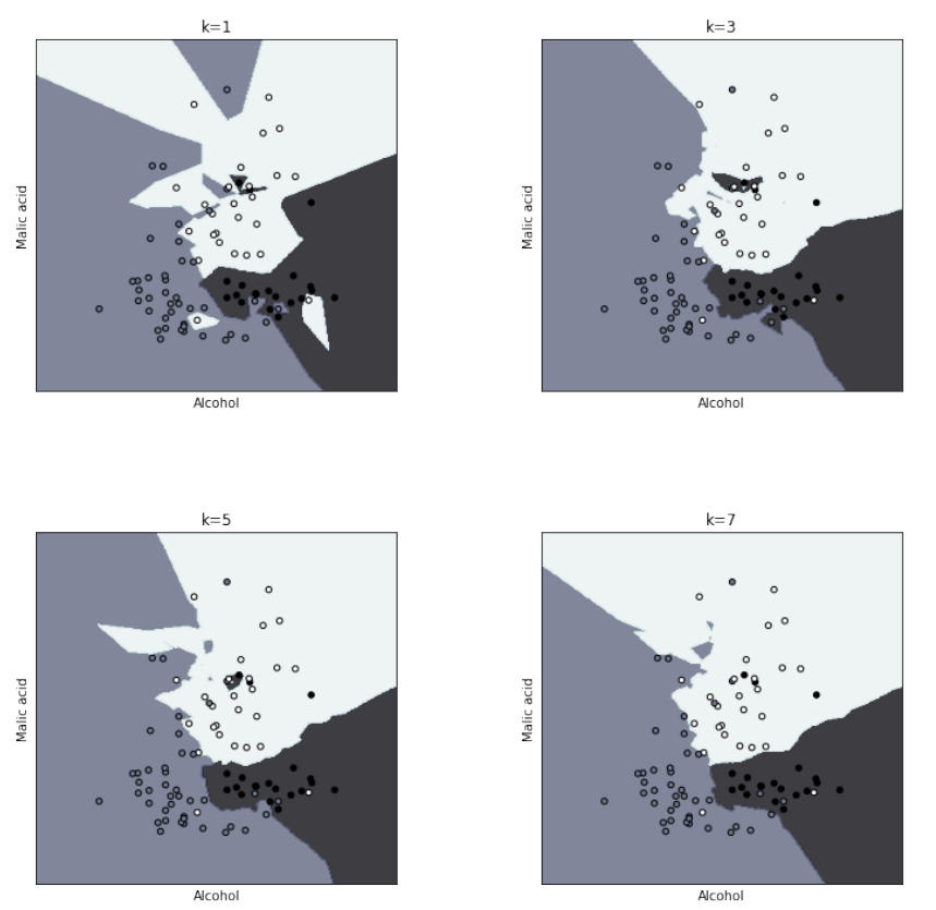
Looking at this image we can infer that for low Ks the boundaries are more serrated, because the classifier is not so aware of the overall distribution and the fit has a low bias, but a high variance. On the contrary, for high Ks the boundaries become really smooth, with a high bias and a low variance (resilience to outliers).

From these results we can see that the decision boundaries are really complex and non-linear, but they reflects well the classes (it is used the Voronoi tessellation to patition the space in regions and the boundary is a set of points at same distance from two different training examples). The boundaries changes because of the modification of the Voronoi’s tessellation that, given the set of points and the k, it is fixed for every class.

Model testing

After the best k value is found on the validation set, the model will be used on the test set, that must simulate real world data. An accuracy comparison plot is needed too.

knn = KNeighborsClassifier(n_neighbors=best_k, n_jobs=-1)
knn.fit(X_trainval, y_trainval)

test_score = knn.score(X_test, y_test)
predictions = knn.predict(X_test)

print('Prediction accuracy on test set for k=' + str(best_k))
print('{:.2%}\n'.format(test_score))
print('report: \n' + classification_report(y_test, predictions))

` Prediction accuracy on test set for k=7 -> 81.48% `

The main problem of the k-NN is the computational complexity in space and time, especially for big sets, that’s because some approximate versions are really used. For what concerns the evaluation of the model on the test set, it is good. We evaluate with the validation only on the 20% of the data, so the samples are not enough. Moreover, it must be recalled that dataset has been prepared (in the preprocessing stage) and from the f1 in the report the cuttings on the other features cause lacks of informations regarding the class_2.

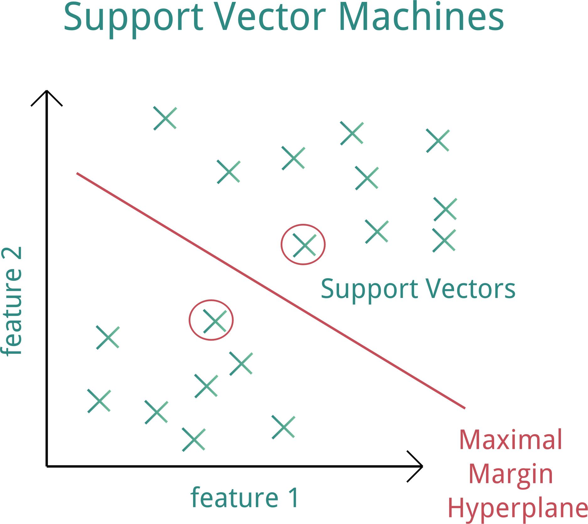
Linear SVM: C tuning

Model training and evaluation

As we already have done with the K-nn, we will train and evaluate one model for each value of C in our hyperparameter list:

[0.001, 0.01, 0.1, 1, 10, 100, 1000]

We want to choose the “C” that gives the highest accuracy when predicting the labels of the evaluation set. If more than one C gives the same accuracy, we choose the lowest C, so the one that gives the larger margin. To train the models we instantiate a SVM for each C and we fit on the train set. At the same time we use the model to predict on the validation set and we save everything in a data structure and, using a personal library, we plot the seven models with the decision boundaries.

…

Download the report to continue reading.